Bayesian information criterion

In statistics, the Bayesian information criterion (BIC) or Schwarz criterion (also SBC, SBIC) is a criterion for model selection among a finite set of models. It is based, in part, on the likelihood function, and it is closely related to Akaike information criterion (AIC).

When fitting models, it is possible to increase the likelihood by adding parameters, but doing so may result in overfitting. The BIC resolves this problem by introducing a penalty term for the number of parameters in the model. The penalty term is larger in BIC than in AIC.

The BIC was developed by Gideon E. Schwarz, who gave a Bayesian argument for adopting it.^[1] It is closely related to the Akaike information criterion (AIC). In fact, Akaike was so impressed with Schwarz's Bayesian formalism that he developed his own Bayesian formalism, now often referred to as the ABIC for "a Bayesian Information Criterion" or more casually "Akaike's Bayesian Information Criterion".^[2]

1 Mathematically
2 Characteristics of the Bayesian information criterion
3 Applications
4 See also
5 Notes
6 References
7 External links

Mathematically

The BIC is an asymptotic result derived under the assumptions that the data distribution is in the exponential family. Let:

x = the observed data;
n = the number of data points in x, the number of observations, or equivalently, the sample size;
k = the number of free parameters to be estimated. If the estimated model is a linear regression, k is the number of regressors, including the intercept;
p(x|k) = the probability of the observed data given the number of parameters; or, the likelihood of the parameters given the dataset;
L = the maximized value of the likelihood function for the estimated model.

The formula for the BIC is:^[3]^[4]

${-2 \cdot \ln{p(x|k)}} \approx \mathrm{BIC} = {-2 \cdot \ln{L} %2B k \ln(n) }. \$

Under the assumption that the model errors or disturbances are independent and identically distributed according to a normal distribution and that the boundary condition that the derivative of the log likelihood in respect to the true variance is zero, this becomes (up to an additive constant, which depends only on n and not on the model)^[5]:

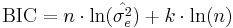
$\mathrm{BIC} = n \cdot \ln(\hat{\sigma_e^2}) %2B k \cdot \ln(n) \$

where $\hat{\sigma_e^2}$ is the error variance.

The error variance in this case is defined as

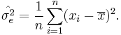
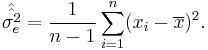
$\hat{\sigma_e^2} = \frac{1}{n} \sum_{i=1}^n (x_i-\overline{x})^2.$

One may point out from probability theory that $\hat{\sigma_e^2}$ is a biased estimator for the true variance, $\sigma^2$ . Let $\hat{\hat{\sigma_e^2}}$ denote the unbiased form of approximating the error variance. It is defined as

$\hat{\hat{\sigma_e^2}} = \frac{1}{n-1} \sum_{i=1}^n (x_i-\overline{x})^2.$

Additionally, under the assumption of normality the following version may be more tractable

$\mathrm{BIC}= \chi^2 %2B k \cdot \ln(n). \,$

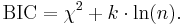
Note that there is a constant added that follows from transition from log-likelihood to ${\chi}^{2}$ ; however, in using the BIC to determine the "best" model the constant becomes trivial.

Given any two estimated models, the model with the lower value of BIC is the one to be preferred. The BIC is an increasing function of $\sigma_e^2$ and an increasing function of k. That is, unexplained variation in the dependent variable and the number of explanatory variables increase the value of BIC. Hence, lower BIC implies either fewer explanatory variables, better fit, or both. The BIC generally penalizes free parameters more strongly than does the Akaike information criterion, though it depends on the size of n and relative magnitude of n and k.

It is important to keep in mind that the BIC can be used to compare estimated models only when the numerical values of the dependent variable are identical for all estimates being compared. The models being compared need not be nested, unlike the case when models are being compared using an F or likelihood ratio test.

Characteristics of the Bayesian information criterion

It is independent of the prior or the prior is "vague" (a constant).
It can measure the efficiency of the parameterized model in terms of predicting the data.
It penalizes the complexity of the model where complexity refers to the number of parameters in model.
It is approximately equal to the minimum description length criterion but with negative sign.
It can be used to choose the number of clusters according to the intrinsic complexity present in a particular dataset.
It is closely related to other penalized likelihood criteria such as RIC and the Akaike information criterion.

Applications

BIC has been widely used for model identification in time series and linear regression. It can, however, be applied quite widely to any set of maximum likelihood-based models. However, in many applications (for example, selecting a black body or power law spectrum for an astronomical source), BIC simply reduces to maximum likelihood selection because the number of parameters is equal for the models of interest.

Notes

^ Schwarz, Gideon E. (1978). "Estimating the dimension of a model". Annals of Statistics 6 (2): 461–464. doi:10.1214/aos/1176344136. MR 468014.
^ Akaike, H., 1977. "On entropy maximization principle". In: Krishnaiah, P.R. (Editor). Applications of Statistics, North-Holland, Amsterdam, pp. 27–41.
^ http://arxiv.org/PS_cache/astro-ph/pdf/0701/0701113v2.pdf
^ http://nscs00.ucmerced.edu/~nkumar4/BhatKumarBIC.pdf
^ Priestley, M.B. (1981) Spectral Analysis and Time Series, Academic Press. ISBN 0-12-564933-3 (p. 375)

References

Liddle, A.R., "Information criteria for astrophysical model selection", http://arxiv.org/PS_cache/astro-ph/pdf/0701/0701113v2.pdf
Bhat, H. S. and Kumar, N., "On the derivation of the Bayesian Information Criterion", http://nscs00.ucmerced.edu/~nkumar4/BhatKumarBIC.pdf
McQuarrie, A. D. R., and Tsai, C.-L., 1998. Regression and Time Series Model Selection. World Scientific.

External links

Information Criteria and Model Selection